Inter-rater reliability in behavioural coding: a practical guide to Cohen's kappa

Inter-rater reliability is the evidence that a coding scheme measures behaviour, not the coder. In observational research, every conclusion rests on how video and audio are coded — so reviewers and readers need to know that two trained people, working independently, would assign the same codes to the same moments. This guide explains what inter-rater reliability is, how Cohen's kappa quantifies it, how to read it honestly, where it misleads, and how to report it — drawing on the methods literature rather than on rules of thumb.

What is inter-rater reliability?

Inter-rater reliability (IRR) is the degree to which independent coders assign the same codes to the same behaviour. It is what separates a reproducible coding scheme from one person’s idiosyncratic interpretation. The measuring instrument in observational research is a trained human applying a coding scheme, so — as with any instrument — its accuracy has to be established before the data carry weight (Bakeman, Deckner & Quera, 2005). If a second coder, blind to the first, reaches the same decisions, the scheme is doing the work; if not, the results may reflect a judgement rather than the phenomenon.

IRR is not a formality. It is one of the first things peer reviewers check in any observational study, because every downstream statistic inherits the reliability of the coding beneath it.

What is Cohen’s kappa?

Cohen’s kappa (κ) is a statistic that measures agreement between two coders while correcting for the agreement expected by chance (Cohen, 1960). It is an overall summary statistic (an omnibus statistic, in the methods literature) — a single number that summarises a whole table of agreements and disagreements. It answers a sharper question than “how often did the coders agree?”: “how much did they agree beyond what chance alone would have produced?”

The formula is straightforward:

κ = (pₒ − pₑ) / (1 − pₑ)

where pₒ is the observed proportion of agreement and pₑ is the proportion expected by chance, given how often each code is used. Kappa runs from 1 (perfect agreement) through 0 (chance-level) and can go negative when coders agree less often than chance would predict — which usually signals systematic disagreement or a data-entry error.

Why percentage agreement is not enough

Raw percentage agreement overstates reliability because it ignores chance. Take a behaviour that is present 90% of the time. If two coders do not truly judge each moment but simply guess in line with that base rate — each choosing “present” 90% of the time and “absent” 10% — they will still agree through frequency alone: 0.90 × 0.90 = 81% of the time on “present”, plus 0.10 × 0.10 = 1% on “absent”, which is roughly 82% in total. That 82% is pure chance; no one actually evaluated the material. Percentage agreement would call it excellent, whereas Cohen’s kappa removes exactly this chance component. If observed agreement were also 82%, then κ = (0.82 − 0.82) / (1 − 0.82) = 0 — correctly showing no agreement beyond chance. Correcting for chance is the whole point of using kappa rather than a simple agreement rate.

The agreement matrix is where the real information lives

A kappa value is computed from an agreement matrix — also called a confusion matrix or kappa table. Rows are one coder’s decisions, columns the other’s, and both are labelled with the same set of mutually exclusive, exhaustive codes. Agreements fall on the diagonal; every off-diagonal cell is a specific disagreement (Bakeman, Deckner & Quera, 2005). The single kappa number hides all of this, yet the matrix is where the useful, actionable information sits.

Two patterns are worth reading directly off the matrix:

• Symmetric versus asymmetric disagreements. If coder A calls something “fuss” that coder B calls “cry” about as often as the reverse, the disagreement is symmetric — the two are equally, mutually confused. If the swaps run mostly one way (A keeps coding “cry” where B codes “fuss”, but rarely the reverse), the disagreement is asymmetric, which means the coders are applying different thresholds for that code. Asymmetric disagreements are the more serious of the two: they point to a calibration problem that retraining can fix.
• Which codes cause the trouble. Because kappa is a single overall figure, it does not tell you which distinctions were hard. Computing a separate kappa for each code (a 2 × 2 table per code) identifies the problematic ones, and the off-diagonal cells show exactly which pairs of codes coders confuse (Bakeman, 2022).

In short: report the overall kappa, but diagnose with the matrix.

”Is kappa big enough?” is the wrong question

A familiar set of interpretive benchmarks comes from Landis and Koch (1977): below 0 poor, 0.00–0.20 slight, 0.21–0.40 fair, 0.41–0.60 moderate, 0.61–0.80 substantial, 0.81–1.00 almost perfect. Fleiss (1981) offered a similar scheme. These labels are convenient, but they were not supported by a strong rationale, and — more importantly — they ignore the circumstances that drive the value of kappa (Bakeman, 2022).

The deeper problem is that no single value of kappa is universally acceptable, because kappa depends on more than how accurate the coders were. Bakeman and Quera (2011) list the circumstances that shift it: observer accuracy, the number of codes, the prevalence of each code, observer bias (a difference in how the two coders distribute their codes), and observer independence. Two of these matter a great deal:

• The number of codes. When a scheme has fewer than five codes — especially with skewed prevalence — equally accurate observers will produce a lower kappa. With more than five codes, the number of codes and prevalence variability matter little. So a kappa of .61 from a two-code scheme is not the same achievement as a kappa of .61 from an eight-code scheme.
• Prevalence. When one code is very common or very rare, kappa can be surprisingly low even when coders agree on almost every event — the so-called prevalence paradox.

Because of this, a lone kappa is almost impossible to interpret. Bakeman (2022) recommends turning the question around: ask not “is kappa big enough?” but “are the observers accurate enough?” His KappaAcc method estimates the observer accuracy that simulated coders would need to reproduce the observed kappa, given the actual number of codes and base rates. In one worked example, an overall kappa of .61 (69% raw agreement) across five codes corresponded to about 82% observer accuracy — below a typical target of 85%. Accuracy is intuitive in a way that a bare kappa is not, and it makes “good enough” a deliberate, statable standard rather than a borrowed cut-off.

Kappa maximum: when the marginals cap the score

Kappa can reach 1 only when both coders distribute their codes identically — that is, when the row and column totals (the marginals) match. When they differ, the maximum value kappa could attain falls below 1, and the more discrepant the marginals, the lower that ceiling (Bakeman, Deckner & Quera, 2005). In one example, an observed kappa of .74 sat against a kappa maximum of .87 — so the coders reached 85% of what was achievable given how they distributed their codes. A modest-looking kappa of .58 in another table reached 87% of its maximum of .67.

Reporting kappa against its maximum can therefore put a “low” value in fairer perspective. But it is not a rescue device: a low kappa maximum is itself produced by discrepant marginals, which usually means asymmetric disagreement — a calibration problem worth investigating rather than explaining away. As Bakeman and colleagues put it, kappa maximum is no panacea for low kappas.

Two kinds of disagreement: quantity and allocation

A useful way to think about why coders disagree comes from accuracy assessment in map comparison, where Pontius and Millones (2011) argue — in a paper pointedly titled “Death to Kappa” — that a single chance-corrected index obscures more than it reveals. They recommend decomposing total disagreement into two interpretable parts:

• Quantity disagreement — disagreement about how much: the two sources differ in the overall proportion assigned to a category. In coding terms, this is a difference in marginals — one coder simply uses a code more often than the other.
• Allocation disagreement — disagreement about which: even when the proportions match, the two differ on which specific events receive which code.

The lesson transfers cleanly to behavioural coding. “Quantity” disagreement is essentially observer bias and the marginal mismatch that lowers kappa maximum; “allocation” disagreement is genuine, event-by-event confusion about category membership. Separating the two tells you what to fix: a quantity problem calls for recalibrating thresholds, while an allocation problem calls for sharper code definitions or more training on hard cases. Pontius and Millones go further and argue that kappa adds little beyond plain proportion agreement for practical decisions; one need not accept the full “abandon kappa” position to take the constructive point — read the disagreement, don’t just chance-correct it.

Coding on a timeline: segmentation, time-unit kappa and the tolerance window

The simple picture of kappa assumes the units are already segmented — coders just sort pre-cut events like billiard balls by colour. Real behavioural coding is usually a two-fold task: coders must both find the boundaries between behaviours and classify what lies between them (Bakeman, Deckner & Quera, 2005). Disagreement can therefore arise from boundary placement as much as from category choice.

A robust solution is to compute kappa on time units — for example, treating each second as the thing coded. A second-by-second agreement matrix captures both aspects of the task at once: where the boundaries fell and which code applied. The trade-off is that two coders will almost never mark a boundary at exactly the same instant, so exact-second matching would understate real agreement.

This is what the tolerance window (sometimes called slippage) is for: a second counts as agreement if the other coder assigned the same code within a defined window. Setting slippage to ±2 seconds, for instance, accepts agreement anywhere in a five-second span. The window is part of the method and must be reported, because a wider window will, all else equal, raise agreement. Good tools also plot a timeline of disagreements, showing exactly where in the session coders diverged — which is invaluable for reviewing the recording and targeting retraining (Bakeman, Deckner & Quera, 2005).

What you code shapes how reliably you can code it

A coder’s skill is only part of the story. The behaviour itself — how long it lasts, how often it occurs, and how clearly it can be recognised — sets much of the ceiling on achievable agreement, independently of training.

Duration. Behaviours fall on a spectrum from momentary events, whose timing but not length is of interest (a pointing gesture, a head-turn), to duration events or states that persist (a play episode, a feeding bout) (Bakeman, Deckner & Quera, 2005). On a second-by-second timeline, a long state accumulates many agreeing seconds, so a one- or two-second disagreement about exactly where it begins or ends is a small fraction of the whole and barely moves kappa. A brief momentary event is the opposite case: a boundary discrepancy of a second or two can be the entire event, so the tolerance window does much heavier lifting and the chosen window size strongly shapes the result. The shorter the behaviour, the more carefully the match window has to be justified and reported.

Frequency. Rare codes are doubly disadvantaged. They offer few opportunities for agreement, and on a time base they occupy very few “present” seconds among a sea of “absent” ones — the prevalence skew that can depress kappa even when coders agree on nearly every actual occurrence. For rare, brief behaviours, an event-based agreement check or a per-code kappa often tells a fairer story than the overall time-unit figure alone.

Identifiability. Some behaviours are intrinsically harder to spot than others. A grasp, a point or a change of position is discrete and visible; a fleeting eye-roll, a subtle shift of affect or a direction of gaze is ambiguous and easy to miss or to read differently. This is not a failure of training — it is a property of the behaviour. Gardner (cited in Bakeman, 2022) noted that around 80% observer accuracy, modest as it sounds, may be representative for some social behaviours and expressions of affect. The practical consequence reinforces the central theme of this guide: a realistic reliability target should be set per behaviour rather than borrowed as a single cut-off, and subtle codes need especially sharp operational definitions, anchor examples and calibration before data collection begins.

Taken together, these three properties are why a per-code kappa, read off the agreement matrix, is so informative: it shows which behaviours the scheme can capture reliably and which are inherently fragile — information a single overall value hides.

How much data should you double-code?

There is no universal rule, but a widely used convention is to have a second coder independently re-code a representative subset — often around 15–20% of the material — and to report inter-rater reliability on that subset. State explicitly how much was double-coded and how the subset was selected, so that reviewers can judge whether the estimate is representative of the full dataset.

Reliability is not a one-off number

Establishing reliability serves two distinct purposes, one at each end of a project (Bakeman, Deckner & Quera, 2005). During training, kappa gives novice coders a clear target, while the agreement matrix and timeline plots show what to retrain — which codes are confused and where. During data collection, periodic reliability checks confirm that coders are still coding consistently; a drifting kappa is an early warning that definitions have slipped and recalibration is due. Treating reliability as a single number computed once, purely for the methods section, throws away its most useful function: keeping the measuring instrument calibrated over the life of the study.

Common pitfalls

• Reporting a lone kappa. Without the number of codes, the number of tallies and the base rates, a single kappa is almost uninterpretable (Bakeman, 2022).
• Treating the benchmark as a verdict. A value of 0.79 is not a failure and 0.81 is not a triumph; the bands are smooth heuristics, not cliffs.
• The prevalence paradox. With very skewed base rates, kappa can be low despite near-total agreement. Report prevalence, and where it is extreme consider complementary indices (for example, prevalence- and bias-adjusted kappa).
• Coders who are not truly independent. If coders confer while coding the reliability subset, the estimate is inflated. Reliability coding must be blind and independent.
• Leaning on kappa maximum to excuse a low kappa. A low ceiling usually reflects asymmetric disagreement that deserves scrutiny, not a footnote.

How to report inter-rater reliability

A complete report states, at minimum: which behaviours were assessed and how the scheme defined them; how much material was double-coded and how the subset was chosen; the tolerance window used for timeline data; the number of codes and the number of tallies in the kappa table; the reliability statistic and its value for each code; and the software used (Bakeman, 2022). Reporting kappa per code — rather than a single pooled figure — lets readers see which distinctions were easy and which were hard, and stating the number of codes and base rates lets them interpret the value at all.

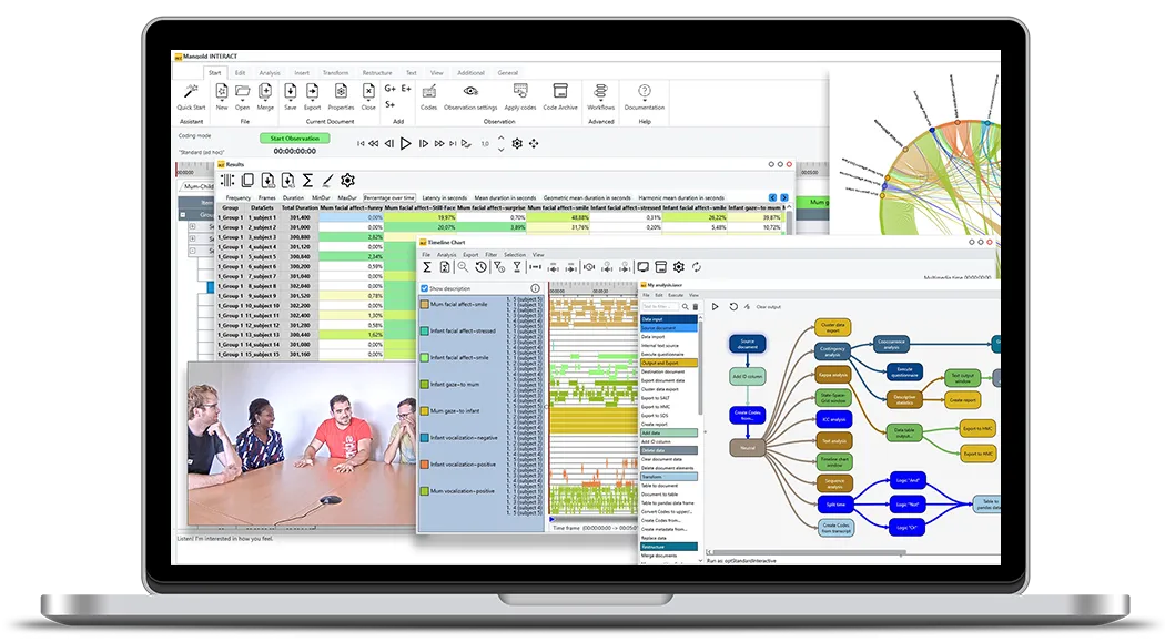
How Mangold INTERACT handles inter-rater reliability

Mangold INTERACT computes Cohen’s kappa directly from two independently coded timelines, and it turns the two decisions this guide has flagged as decisive — what counts as a match, and how time is handled — into explicit, adjustable parameters rather than hidden defaults. Its own manual is candid that these settings can strongly influence the resulting kappa, and that there is no universally best configuration, because the right values depend on the type of codes, the length of the events and the accuracy required — the same point made above about duration and identifiability.

The matching parameters. Two criteria define agreement. The overlap percentage sets, for codes that have a duration, how much two events must overlap in time to count as a match; because long states overlap easily and brief events barely do, the manual advises lowering the overlap requirement when codes are short — exactly the duration effect described earlier. The tolerance window handles very short events that may not overlap at all: a time value defines how close the two start times must be for the codes to count as a match. This is the slippage window of timeline coding, and when a lot happens in a short span the manual recommends shrinking it so as not to inflate agreement. The same two criteria, with their own values, are then applied to flag mismatches — different codes that align in time — so that the procedure builds the full agreement-and-disagreement picture rather than counting hits alone.

The pair-finding routine. INTERACT resolves the two timelines into pairs in a defined order, comparing only codes within matching datasets, so one subject’s coding is never matched against another’s. Simplified, it first links identical codes that overlap in time (agreements), then links identical codes whose start times fall within the tolerance window (agreements for short events), then links differing codes that fall within the window (disagreements), and finally leaves anything still unmatched as a “No Pairs” entry — counted as “observer A coded something where observer B coded nothing”. Those “No Pairs” cases are precisely the omission-and-commission disagreements that lower kappa, surfaced explicitly rather than buried. The whole routine can be stepped through one decision at a time, with the parameters used at each stage shown beneath the diagram, so a reviewer can audit exactly how each pair was formed.

Reading the result. The outcome appears as a colour-coded kappa graph and an agreement matrix: matches on the diagonal, mismatches in red, and unmatched codes in the “No Pairs” row and column. INTERACT can compare two coders, one coder against several others, or all coders against each other — supporting both classic two-rater checks and multi-rater designs. Because the matrix and the timeline of pairs are visible, reliability in INTERACT is a diagnostic tool, not just a single number: it shows which codes were confused and where, which is what turns a reliability check into targeted feedback for retraining. The software does not replace a well-defined coding scheme or the judgement behind it — but it makes every consequential setting explicit, reportable and auditable.

Reading INTERACT’s kappa results — and avoiding the common traps

INTERACT presents the result as a per-class agreement matrix — matched pairs on the diagonal, mismatches off it — with a per-code percentage agreement alongside P(observed) and P(expected). The kappa value, the number of codings, the file names compared and the exact parameters used are all recorded with the output, so a result is reproducible and auditable. A handful of recurring situations are worth knowing, most of them properties of Cohen’s kappa rather than of the software:

• A kappa near zero or negative usually means too little to work with. Kappa is probability-based and needs a pool of distinct codes, so a class with only one or two codes, or a dataset with very few events, cannot produce a meaningful value — and a kappa of exactly zero means observed agreement equalled chance agreement. The fixes are to pool more material (merge each observer’s sessions into one compilation file before computing), to make a sparse class gap-free by filling gaps with a neutral placeholder code (which raises the number of codes per class), or to combine several classes into one.
• There is no single “overall kappa” across classes. Cohen defined kappa per mutually exclusive, exhaustive class, so INTERACT reports it per class; if you need one figure, you deliberately combine the relevant codes into a single class and read that.
• INTERACT reports a per-code percentage agreement, not a per-code kappa. The percentage is offered for coding systems that kappa does not suit, and lets you, for example, compare a trainer’s coding with a trainee’s code by code.
• File order can change the result. Because a match depends on how much two events overlap, an 80% overlap requirement is easier to satisfy against a longer event than a shorter one, so swapping which file is the “master” can flip a borderline pair. Report the comparison order and the parameter values along with kappa.
• Kappa ignores things you may care about. It does not weight how hard a behaviour is to code, the semantics of a code, or the variance in event durations — the same limitations discussed above. This is exactly why the parameters and the matrix should be reported and read, not just the headline number.

How the overlap threshold plays out — a worked example. Suppose the “master” file codes behaviour A for 4 seconds, while the second file codes the same behaviour A for 8 seconds at roughly the same moment, slightly offset. With an 80% overlap requirement, 80% of the 4-second event is 3.2 seconds — comfortably contained in the 8-second event, so the pair is counted as a match. Swap the file order and the threshold is now taken against the 8-second event: 80% of 8 seconds is 6.4 seconds, which a 4-second event can never cover, so the overlap rule on its own would record a mismatch. Here the tolerance window acts as a safety net — if no other event competes and the shorter event begins within the window measured from the start of the longer one, INTERACT still records a match. The practical takeaway: for events of uneven length, choose the overlap percentage with the shorter event in mind, rely on the tolerance window, and report both the parameter values and which file served as the master.

A worked example from infant-development research

A recent open-access study illustrates good practice. Kaletsch and Liszkowski (2026, Journal of Cognition and Development) tested whether training caregivers to respond more to their infants increased 12-month-olds’ index-finger pointing. The team coded infants’ pointing gestures and caregivers’ responsiveness from video, double-coded 20% of the recordings with a two-second match window, and reported Cohen’s kappa per code: κ = .82 for infants’ index-finger points, .81 for caregivers’ responsiveness, and .88 for caregivers’ points — all in the “almost perfect” range. Only after establishing that reliability did the authors report their behavioural findings. That ordering — reliability first, results second, and reported per code with the match window stated — is exactly what makes the results credible.

Key takeaways

• Inter-rater reliability shows that a coding scheme is reproducible, not idiosyncratic.
• Cohen’s kappa is preferred over percentage agreement because it corrects for chance.
• A lone kappa is hard to interpret: its value depends on the number of codes and the base rates, so report those alongside it.
• Ask “are observers accurate enough?” rather than “is kappa big enough?”; estimated observer accuracy is more intuitive than a borrowed cut-off.
• Diagnose with the agreement matrix: symmetric versus asymmetric disagreements, per-code kappas, and kappa maximum where marginals are discrepant.
• For timeline coding, compute kappa on time units, report the tolerance window, and use timeline plots to target retraining.
• The behaviour itself — its duration, frequency and how hard it is to spot — sets much of the achievable agreement; set reliability targets per behaviour and read per-code kappas.
• Double-code a representative subset (commonly ~15–20%), and treat reliability as ongoing calibration, not a one-off number.

INTERACT: One Software for Your Entire Observational Research Workflow

From audio/video-based content-coding and transcription to analysis - INTERACT has you covered.

Explore INTERACT

References and further reading

• Bakeman, R. (2022). KappaAcc: A program for assessing the adequacy of kappa. Behavior Research Methods, 55, 633–638.
• Bakeman, R., Deckner, D. F., & Quera, V. (2005). Analysis of behavioral streams. In D. M. Teti (Ed.), Handbook of Research Methods in Developmental Psychology. Blackwell.
• Bakeman, R., & Quera, V. (2011). Sequential analysis and observational methods for the behavioral sciences. Cambridge University Press.
• Cohen, J. (1960). A coefficient of agreement for nominal scales. Educational and Psychological Measurement, 20(1), 37–46.
• Fleiss, J. L. (1981). Statistical methods for rates and proportions. Wiley.
• Landis, J. R., & Koch, G. G. (1977). The measurement of observer agreement for categorical data. Biometrics, 33(1), 159–174.
• Pontius, R. G., & Millones, M. (2011). Death to Kappa: birth of quantity disagreement and allocation disagreement for accuracy assessment. International Journal of Remote Sensing, 32(15), 4407–4429.